Instantaneous Firing Rates

This guide covers how to compute instantaneous firing rates from spike trains, project them into low-dimensional manifolds, and work with the RateData class. For pairwise firing-rate correlations, see the Pairwise Analysis guide.

All examples assume you already have a SpikeData object loaded. See the Quick Start for how to create one.

from spikelab import SpikeData, RateData

Instantaneous Firing Rates

Mean firing rates (sd.rates()) give one number per unit, but many analyses require a time-resolved estimate. SpikeLab provides two methods for computing per-unit instantaneous firing rate traces, both returning a RateData object.

ISI interpolation

resampled_isi() estimates the instantaneous rate by interpolating the inverse inter-spike interval at a set of time points and smoothing with a Gaussian kernel:

import numpy as np

# Define the time grid (e.g. every 1 ms across the recording)
times = np.arange(0, sd.length, 1.0)

rd = sd.resampled_isi(
    times,
    sigma_ms=10.0,   # Gaussian smoothing kernel width (ms)
)
# rd.inst_Frate_data.shape == (sd.N, len(times))

Sliding window

sliding_rate() computes rates by counting spikes in a centered sliding window and dividing by the window width. Both the sliding-window step and an additional Gaussian smoothing step are optional and can be used independently or in combination:

rd = sd.sliding_rate(
    window_size=50,       # sliding window width (ms)
    step_size=1.0,        # advance step (ms)
    gauss_sigma=10.0,     # optional Gaussian smoothing (ms); 0 to disable
    apply_square=True,    # set False to skip the sliding window step
)
# rd.inst_Frate_data.shape == (sd.N, T)

You can also specify sampling_rate instead of step_size (they are mutually exclusive).

Working with RateData

Both methods return a RateData object that carries the rate matrix together with its time axis. RateData supports unit and time subsetting (rd.subset(), rd.subtime()), and provides the correlation and dimensionality-reduction methods described below.

from spikelab import RateData

print(rd.N)                      # number of units
print(rd.inst_Frate_data.shape)  # (N, T)

# Plot raster with firing rate heatmap
fig = sd.plot(
    show_raster=True,
    show_fr_rates=True,
    fr_rates=rd.inst_Frate_data,
)

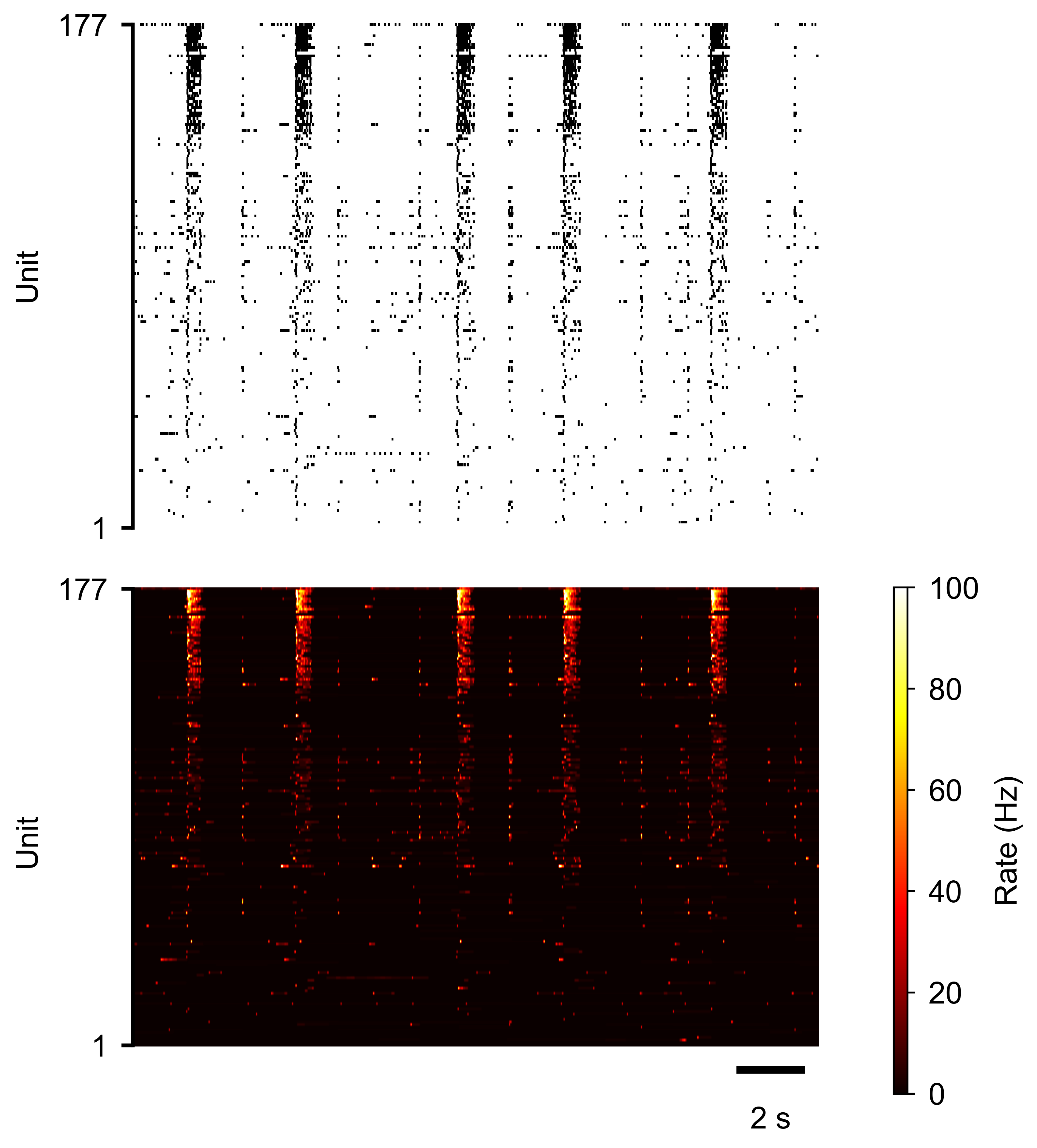
Spike raster with instantaneous firing rate heatmap — Spike raster (top) and instantaneous firing rate heatmap (bottom) for an MEA recording. Each row in the heatmap is one unit; colour intensity reflects firing rate.

Dimensionality Reduction

get_manifold() projects the firing-rate matrix into a low-dimensional space using PCA or UMAP. This is useful for visualising population dynamics over time or comparing activity structure across conditions.

# PCA — returns (embedding, explained_variance_ratio, components)
embedding, var_ratio, components = rd.get_manifold(
    method="PCA",
    n_components=3,
)
# embedding.shape == (T, 3) — one point per time bin

# UMAP — returns (embedding, trustworthiness)
embedding, trust = rd.get_manifold(
    method="UMAP",
    n_components=2,
)

Visualise the embedding with plot_manifold():

from spikelab.spikedata.plot_utils import plot_manifold

fig, ax = plt.subplots(figsize=(5, 5))
plot_manifold(
    ax,
    embedding,
    var_explained=var_ratio,
    groups=condition_labels,       # integer array (T,)
    group_labels=["D0", "D3", "D10", "D30", "D50"],
    marker_size=1,
    alpha=0.3,
)

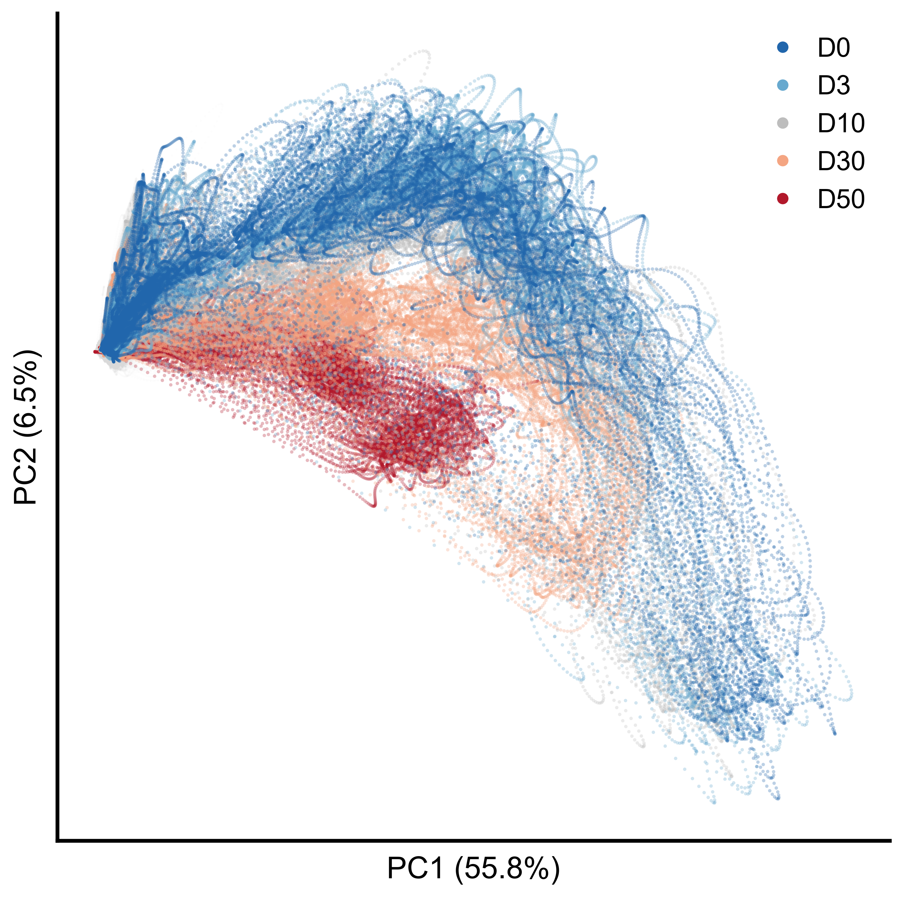
PCA embedding of firing rate dynamics — PCA embedding of instantaneous firing rate dynamics across conditions. Each point is one time bin; colours indicate experimental conditions.

Pairwise Firing-Rate Correlations

Once you have a RateData object, you can compute pairwise correlations between all unit pairs using get_pairwise_fr_corr(). See the Pairwise Analysis guide for full details, code examples, and visualisation of correlation matrices across conditions.

Instantaneous Firing Rates